Sensor Data Pipelines: What Happens Between the Device and the Alert

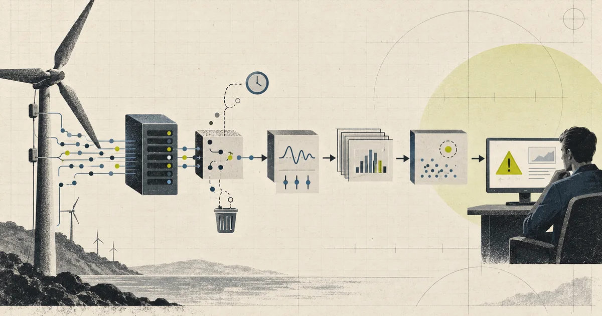
A temperature probe on a motor housing reports twenty-five times a second. A pressure sensor on a hydraulic line does the same. A vibration sensor on a gearbox does it faster.

Nothing about those sensors is unusual. What is unusual is what happens if you treat their output as ordinary application events, because the volume is set entirely by physics rather than by how many people are using the product.

This article walks the path from a sensor reading to an operator’s screen, and spends most of its time on the two places where naive designs break: partitioned state and windowed anomaly detection.

One number decides the design

Take a concrete deployment: vibration monitoring on production equipment, 2,000 sensors sampling at 25 Hz.

2,000 sensors x 25 readings/sec = 50,000 readings/sec

Now the numbers that follow from that.

50,000/sec x 86,400 sec      = 4.32 billion readings per day
4.32 billion x 365 days      = 1.58 trillion readings per year
at ~100 bytes per reading    = 157 TB per year raw

Fifty thousand per second sounds ordinary. Almost every streaming technology handles it without difficulty, and that is exactly why it is a good teaching case. The volume is high enough that a relational table is finished, and low enough that you can reason about the whole design on paper.

The temptation is to treat fifty million per second as the same problem with a bigger number. It is not, and there is a section later in this article about what actually changes. For now, hold the number at fifty thousand and be precise about it.

The 50,000 per second case

At 100 bytes per reading, the wire volume is:

50,000/sec x 100 bytes = 5 MB/sec = 432 GB per day

A week of retention in the log is around 3 TB before compression. Kafka’s batch compression on numeric payloads typically gets that down several times over, which is why compression policy is worth tuning rather than ignoring.

The read side is much smaller. Nobody queries fifty thousand readings per second interactively. What people do is look at a chart, look at an alarm list, and occasionally run a report over a week. That asymmetry is the single most useful fact about a sensor pipeline: the write path is enormous and the read path is tiny.

Design for that. It means the log can be cheap and the query tier can be small, and it means the storage that matters is whatever the alerting and reporting layers keep, not the log itself.

Why the stream needs a log in the middle

The obvious pipeline is device to processor to database. It fails the first time a processor restarts, because the readings that arrived during the restart are gone.

A log in the middle turns a fragile pipeline into a recoverable one.

sensors -> broker (durable, partitioned) -> processor -> sinks
                              |
                              +-> replay from any offset after a failure
                              +-> a new consumer can catch up from scratch
                              +-> backpressure lives in the log, not in the device

Three properties of the broker matter more than its raw throughput.

Retention decides how long you can replay. A seven-day retention means a broken alerting pipeline can be rebuilt from seven days of history instead of from nothing.

Partitioning decides ordering and parallelism. This is the next section and it is the most consequential choice in the design.

Delivery semantics decide what your processor has to handle. Kafka is at-least-once, so the processor sees duplicates, and the sink must be idempotent or the pipeline must deduplicate.

Partitioning decides everything downstream

The partition key is the first thing to get right, because it determines what state is local.

Keying by sensor_id puts all readings for one sensor in one partition. That gives you:

• per-sensor ordering, which matters when consecutive samples are used together;
• all of a sensor’s state in one place, so no cross-partition coordination is needed;
• one alert stream per sensor, free of interleaving.

The cost is that a single partition now carries one sensor’s full rate. At 25 Hz that is nothing. If one very high-rate sensor ever joins the fleet, it becomes a hot partition and the whole pipeline’s throughput is bounded by that one key.

Keying by site_id spreads load better, since a site has many sensors. The cost is that readings for one sensor interleave with others, so a per-sensor rolling window needs state for every sensor in the site on one node.

Neither is wrong. The honest framing is that the key is a statement about where the state lives, and you should make that choice knowing which sensor-level computation you need.

How many partitions? At 50,000 readings per second, a broker that comfortably handles around a million messages per second means 12 partitions is already generous, and 12 gives a natural parallelism for processors.

50,000/sec / 12 partitions = ~4,167 readings/sec per partition

Choose a partition count and then treat it as close to permanent. Adding partitions changes the key-to-partition mapping, which means existing state no longer matches its key. Growing a partitioned stream processor is a real migration, not a config change.

Two paths, not one

A pipeline that writes every reading and evaluates every reading in the same processor has a problem. Alert evaluation needs state and time, and writing raw data needs neither.

Split it.

                     +--> raw path:  write every reading, no state, high volume
broker (sensor topic)|
                     +--> alert path: window, evaluate, emit alarms, lower volume

The raw path is embarrassingly parallel and stateless. It can scale almost linearly with partitions and it never needs to be correct about anything except not losing data.

The alert path is where the state lives, and it is the part that needs careful design. It also processes a small fraction of the volume, because most readings do not need evaluating individually once you have a window.

This split also gives you a place to put quality control. A sensor dictionary, described later, lets the pipeline convert a raw integer into engineering units, and reject readings outside a physically plausible range before they reach anything that cares.

Anomaly detection: threshold and its problems

The simplest rule is a threshold.

if vibration_rms > 8.0 then alarm

It works on the day it is written and it fails within a week, for two reasons.

First, a fixed threshold ignores the fact that a healthy bearing’s vibration depends on speed, load, and temperature. A machine running at a different operating point is legitimately noisier, and the operator learns to ignore the alarm.

Second, a value sitting right at the threshold produces an enormous number of alarms. The reading crosses the line, drops back, crosses again, and you now have a machine with four hundred alarms an hour and no information in any of them.

Both problems are solved by the same two additions.

Deadband and hysteresis

A deadband stops values near the threshold from repeatedly triggering.

enter alarm   if value > 8.0
exit alarm    if value < 7.0

The gap between 7.0 and 8.0 is the hysteresis band. A signal oscillating around 8.0 produces one alarm, not four hundred.

This also gives the operator a genuinely useful distinction: an alarm with a hysteresis band has been sustained, not merely touched.

The deadband should be a property of the rule, not a global constant, because vibration and temperature tolerances have completely different characters. A one-degree band might be noise on a motor bearing and a critical excursion on a coolant line.

Rolling statistics, and the state you just signed up for

Threshold plus deadband still needs a number to compare against, and a fixed number only works if the machine’s normal behaviour never changes.

A rolling baseline fixes that. Keep recent statistics per sensor and compare the current value against its own history.

mean     -> is this reading unusual for this sensor?
stddev   -> how far is unusual, in units of this sensor's normal variation
z-score  = (value - mean) / stddev

A z-score of 3 is a much better alarm than a fixed 8.0, because it adapts to the sensor, the machine, and the operating point.

A fourth option, a rolling range or min-max over the window, catches the slow drifts that a mean and standard deviation miss. Bearings degrade gradually, and a slow upward creep in the standard deviation is an early warning that a fixed threshold will never produce.

Which of these you can afford is entirely a question of state size, and this is where the design usually falls over.

The state size problem

Here is the arithmetic that a stream-processing tutorial tends to skip.

One sensor, a one-week window, 25 Hz:

604,800 seconds x 25 samples = 15,120,000 samples per sensor
2,000 sensors                = 30,240,000,000 samples
at 4 bytes per float         = ~121 GB of state

One hundred and twenty gigabytes of live state, to answer “is this reading unusual”. And that is a single week’s window, held in memory, across the entire fleet.

The problem is not that a stream processor cannot hold a lot of state. The problem is that a window of raw samples has no compression benefit, because a sample’s usefulness is precisely that you did not predict which one you would need.

Three ways out, in increasing order of sophistication.

Keep summary statistics, not samples. Welford’s algorithm maintains a mean and variance in two floats per sensor, in constant space.

2,000 sensors x 2 values x 4 bytes = 16 KB total

That is a reduction of roughly seven million times, and for a mean-and-standard-deviation z-score it loses nothing at all. The weakness is real and worth naming: mean and variance cannot describe a bimodal distribution, so a machine that alternates between two healthy states will look anomalous in both.

Use a sketch. A t-digest or a Greenwald-Khanna quantile summary keeps approximate percentiles in bounded space, typically a few kilobytes per quantile per series.

2,000 sensors x 3 quantiles x ~5 KB = ~30 MB total

That is still a four thousand times reduction, and now you can ask for the 99th percentile of the last week without holding the week. Sketches are approximate, and the approximation error grows with the tail you care about, so validate the accuracy you actually need rather than assuming it.

Downsample before you window. A separate job maintains a 1 Hz or 0.1 Hz series derived from the 25 Hz stream, and the anomaly detector windows the cheap series.

This is the option that scales to fifty million per second, and it has an important limitation: a 0.1 Hz series cannot detect a single-sample spike, because the spike is gone before the downsample sees it. High-frequency faults need a detector running on the raw path, which is why real deployments end up with both a fast stateless rule and a slow statistical model rather than one clever detector.

The practical conclusion is that you should pick your window from the question you need answered, and then check whether the state fits. A one-week rolling window at 25 Hz does not fit. A one-week window at 1 Hz derived from it does.

What changes at fifty million per second

Now the honest section. If the real number is fifty million readings per second rather than fifty thousand, several things stop being adjustable.

Payload becomes the dominant cost. A hundred bytes is no longer viable at that rate, and binary encoding with delta or dictionary compression is not an optimisation but a requirement.

Partition count becomes a design constraint. At a million messages per second per partition, fifty million per second needs at least fifty partitions, and in practice several hundred to survive skew and rebalances.

“Stream processor” stops meaning Flink. At this volume, a stateless map-and-filter over partitions is often the right tool, and a stateful engine is only worth its operational cost where the stateful computation genuinely earns it.

State must be tiny, not merely compact. Anything per-sensor has to be O(1) in space. A twenty-byte sample buffer per sensor at fifty million sensors is already a terabyte of nothing.

Storage is a budget conversation. 50 million per second at 100 bytes is 5 GB per second, which is 432 TB per day. That is not a pipeline you tune, it is a line item.

The design ideas survive the jump. The constants do not. That is the general shape of scaling work, and it is worth internalising before you meet a system that needs it.

Exactly-once, and when you actually need it

Kafka gives at-least-once delivery. A processor that reads a batch, writes to a database, and commits its offset can crash in between and reprocess the batch.

There are three responses, and picking the wrong one is a common and expensive mistake.

Idempotent sink. Give every reading a deterministic identifier, usually sensor id plus timestamp, and make the write a no-op if it already exists. This is the cheapest correct answer and it works for almost every sensor pipeline, because historical readings genuinely are immutable.

Deduplicate in the processor. Keep a window of recently seen identifiers. This is more expensive, it is bounded, and it only covers a recent period, which means it cannot help with a replay from a week ago. Useful as a short-term guard, not as a correctness strategy.

Exactly-once via transactions. Kafka’s transactional producer and consumer API can commit consumed offsets and produced records atomically, which gives exactly-once for Kafka to Kafka. Extending it to an external database means either a distributed transaction coordinator or a two-phase commit, both of which are expensive and both of which have failure modes that are harder to reason about than at-least-once.

The honest position: use at-least-once with an idempotent sink unless you have a specific reason not to. Readings are naturally idempotent, so you have been handed the easy case for free, and trading that away for exactly-once usually costs more than it returns.

Schema and the sensor dictionary

A reading is a number, and on its own a number is nearly useless. Eight thousand is a perfectly plausible bearing temperature and also a perfectly plausible vibration amplitude.

The pipeline needs a sensor dictionary: a registry that maps a sensor id to its meaning.

sensor_id        unit        range          sample_hz   normal   alarm
gearbox-17-temp  degC        0-150          1           62      85
gearbox-17-vib  mm/s RMS    0-50           25          2.1    8.0

This is more important than it looks, for four reasons.

It makes the alerting rules data, not code, so a new sensor does not need a deployment. It makes unit conversion possible at the edge or in the processor instead of in every consumer. It allows plausibility rejection before anything downstream has to defend itself. And it makes the difference between “this sensor is broken” and “this machine is broken” answerable, because a reading outside the dictionary’s range is almost always a broken sensor.

The dictionary is a control-plane entity, and the pipeline is data plane. They should be separate stores, with the pipeline caching the dictionary and refreshing it periodically rather than querying it per reading.

The failure mode to avoid is a dictionary that is quietly out of date, so a rule refers to a sensor that was decommissioned eight months ago and nobody notices because the rule never fires anyway.

Late and out-of-order data

Some readings arrive late, and some arrive in the wrong order. A sensor buffers during a network outage, a cell handover reorders packets, and a partition rebalance interleaves two batches.

Three things to decide.

Allowed lateness. A stream processor will hold a window open until its watermark passes it. Declare how late is acceptable, and what happens beyond that: drop, or accept into a side output for later analysis.

Ordering scope. Ordering exists within a partition. If you key by sensor_id, one sensor’s readings are ordered and the rest of the fleet is independent. That is almost always what you want.

Determinism of updates. If a late reading is lower than a value already written for the same timestamp, decide whether it is ignored or stored. For a temperature sensor, last-arrival-wins is fine. For a cumulative counter, it is a serious bug, because counters only move up and a late low value corrupts the total.

That distinction between a gauge and a counter is worth stating explicitly in your schema, because it changes the deduplication and ordering rules in ways that are painful to discover later.

Backpressure

When the processor cannot keep up, something has to slow down. The choices are to buffer, to shed, or to slow the producer.

Buffer in the log. The broker absorbs the burst and the processor catches up. This works as long as the backlog is measured in minutes. Measured in days, it does not, because the data is now so old that the alert it would have produced is worthless.

Shed load. Downsample or drop readings under pressure. This is the right answer for a high-frequency vibration stream during a spike, and it needs an explicit rule about which data you are willing to lose. Losing 1 Hz derived data is acceptable. Losing the samples needed to diagnose a bearing failure is not.

Slow the producer. Publish a credit or a rate hint that devices can respect. This is rare in sensor networks because the devices are not listening, and a firmware update to make them listen is a multi-quarter project.

The honest statement is that backpressure in a sensor pipeline is a data-quality decision, not just a queueing problem. Deciding in advance that derived data can be dropped and raw data cannot is the useful part.

Failure stories worth testing

Kill a processor mid-window

Restart and confirm the window rebuilds from the log and that no duplicate alarms are emitted for the replayed range. This is the test that proves your log retention and replay story.

Replay a week of history into alerting

If a full replay produces a flood of alarms that nobody would have received live, the rules are not replay-safe. Add a replay flag and suppress notifications, or make the idempotency key include the window.

A sensor starts sending garbage

Full-scale values, or a stuck constant. Confirm plausibility rejection catches it, and that a broken sensor raises a sensor-health alarm instead of being silently discarded.

One partition becomes hot

Add a sensor that reports at 5,000 Hz. Watch per-partition throughput rather than cluster average, which will look fine.

The dictionary changes mid-flight

A sensor is recalibrated and its range narrows. Confirm the processor picks up the change without a restart, and that historical readings are not retroactively judged against the new range.

The broker runs out of disk

Retention is the only thing that frees space. Confirm the pipeline fails visibly rather than accepting writes it will lose.

Clock skew between sensors on the same machine

Two sensors on one gateway with a bad clock produce windows that never align. Use the gateway’s receive time for window assignment and keep the device time as a separate field.

A production-ready architecture

  +----------------+
  | 2,000 sensors  |  25 Hz
  +--------+-------+
           | binary, compressed, batched
           v
  +----------------+     +----------------------+
  | Edge gateway   | --> | Kafka (sensor topic) |
  | validate, tag, |     | 12 partitions        |
  | compress       |     | 7-day retention      |
  +----------------+     +----+------------+----+
                              |            |
                   +----------+            +----------+
                   |                                   |
        +----------v-----------+          +------------v-----------+
        | Raw path             |          | Alert path              |
        | stateless write      |          | keyed by sensor_id      |
        | -> time series       |          | deadband + baseline     |
        | -> object storage   |          | -> alarm service        |
        +----------------------+          +------------+-----------+
                                                          |
                                              +-----------v-----------+
                                              | Notifications, UI     |
                                              +-----------------------+

  Control plane (separate store, cached by pipeline):
  sensor dictionary -> unit, range, sample rate, alarm rules

A sensible delivery checklist:

1. Measure readings per second from physics, and write that number down before choosing a component.
2. Choose the partition key from where state needs to live, not from load spreading alone.
3. Split the stateless raw path from the stateful alert path.
4. Compute the state size for your window before writing the windowed logic.
5. Prefer summary statistics or sketches over raw samples in any stateful detector.
6. Give every rule a deadband, and derive the threshold from a rolling baseline where the machine’s normal range moves.
7. Use at-least-once with an idempotent sink, keyed on sensor id plus timestamp.
8. Declare allowed lateness, and separate gauges from counters in the schema.
9. Keep the sensor dictionary in a control-plane store, cached, and refresh it without a restart.
10. Decide in advance which data may be shed under backpressure and which may not.

Common mistakes

Mistake	What actually happens	Better decision
A rolling window of raw samples	121 GB of state for one week at 25 Hz	Keep summary statistics, a sketch, or a downsampled series
A fixed threshold alarm	A value sitting on the line produces hundreds of alarms an hour	Add a deadband and a rolling baseline
A stateless processor for everything	Windowed logic is spread across all partitions and cannot see a sensor’s history	Separate the stateful alert path
Keying by site to spread load	A per-sensor window now needs state for every sensor on one node	Accept a hot partition, or use sub-keying
Changing partition count later	The key-to-partition mapping changes and state no longer matches	Provision partitions for the next order of magnitude
Exactly-once everywhere	Transactions and coordination cost more than the duplicates you were avoiding	At-least-once with an idempotent sink on sensor id plus timestamp
Treating gauges and counters alike	A late low value corrupts a cumulative total	Declare the metric type and write the ordering rules to match
A bare number on the wire	Eight thousand is a plausible temperature and a plausible amplitude	Carry a sensor dictionary with units, ranges, and rules
Trusting cluster average throughput	One hot partition is invisible in the average	Watch per-partition and per-key throughput
Buffering backpressure in the log	The backlog becomes so old the alarms it would raise are worthless	Shed derived data explicitly, and never raw data
A dictionary nobody updates	Rules reference decommissioned sensors and never fire	Make the dictionary a versioned control-plane entity
Assuming replay is free	A week of replay floods alerting with alarms nobody would have received	Make rules replay-aware, and suppress notification on replay

The complete story in one minute

A sensor samples twenty-five times a second and sends a compact binary reading. An edge gateway validates the shape against the sensor dictionary, tags it with the gateway’s receive time, and publishes it to a Kafka topic partitioned by sensor id, which keeps all of one sensor’s state on one node and gives per-sensor ordering.

Two consumers read that topic. The raw path is stateless and writes every reading to time-series storage and to object storage for long-term analysis. The alert path keeps bounded per-sensor state: a mean and variance for a rolling z-score, optionally a t-digest for percentiles, and a deadband so a value near the threshold raises one alarm rather than hundreds. It never holds a week of raw samples, because that would be a hundred and twenty gigabytes.

Delivery is at-least-once, and the sink deduplicates on sensor id plus timestamp, which is cheap because a historical reading genuinely is immutable. Windows have a declared lateness, and a reading that arrives after the watermark goes to a side output rather than silently mutating history.

If the processor falls behind, the log absorbs a short burst and the pipeline sheds derived data under sustained pressure. Raw samples are never shed, because they are the only version of the data that can diagnose a high-frequency fault later.

That is the whole path:

sample -> validate -> broker -> (raw history | bounded-state alerting) -> alarm

The hard parts were never the throughput. They were keeping the state bounded, making a threshold that survives contact with a real machine, and being honest that a rolling window of raw samples was never going to fit.

What this team still owns

Every derived signal needs its source sensor, calibration/unit metadata, event-time policy, algorithm version, warm-up state, and quality flags. A threshold crossing is not automatically an incident: debouncing, hysteresis, minimum duration, missing-data behaviour, and reset conditions belong in the contract. Bound state by time or count and test replay with late, duplicated, reset, and gapped sequences so recovery produces the same alarms—or an explicitly documented correction.

Technical references

• OGC SensorThings API
• OPC UA Part 8: Data Access
• Apache Flink: event time and watermarks