How a Time-Series Database Stores Data: A Prometheus-Style Design

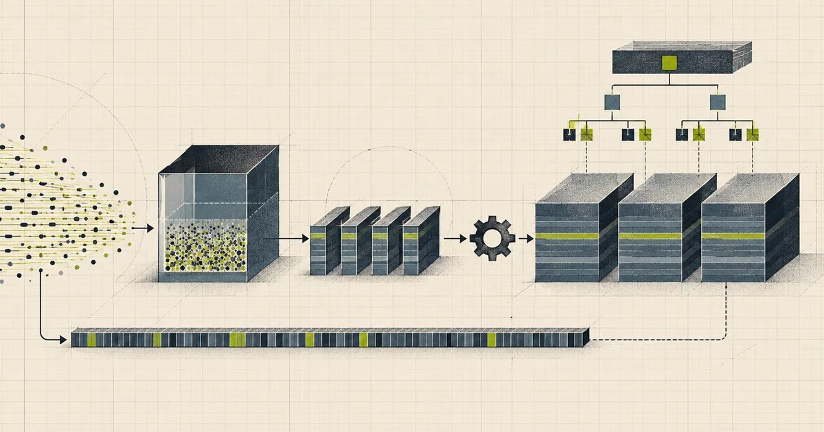
A time series database looks like a simple idea. Rows arrive with a timestamp and some values, you ask for a range, and you get the range back. The implementation is where the design shows itself.

The useful mental model is not “a fast table.” It is a storage design optimized around time-bounded reads and batches of samples from the same series. This article follows a Prometheus/Gorilla-style design because it is concrete; a PostgreSQL/Timescale hypertable, an Influx engine, and a distributed remote store do not share every structure below.

The shape of the data

Take a concrete example: one factory, 100,000 sensors, one reading per second per sensor.

100,000 series
1 sample per second per series
100,000 points per second
8.64 billion points per day

Over a year that is about 3.15 trillion points. This is the shape that matters:

• a bounded set of series, each identified by a small number of labels;
• a mostly append-oriented write path, with an explicit policy for late, duplicate, corrected, and out-of-order samples;
• a time-bounded read path, because nobody queries all of history at once;
• a low cardinality label set, because the whole design depends on it.

Almost every optimisation below follows from those four properties. When a workload does not have them, a time series database is usually the wrong tool, and it is worth saying so early.

Why a relational table gets uncomfortable

The obvious schema is a table with a timestamp and some values.

CREATE TABLE readings (
    sensor_id   uuid        NOT NULL,
    recorded_at timestamptz NOT NULL,
    value       double precision NOT NULL,
    site_id     uuid        NOT NULL
);

This works. It also stores every point twice, because the index and the heap both carry the same information.

heap row  -> sensor_id (16) + recorded_at (8) + value (8) + site_id (16) = 48 bytes
index     -> sensor_id (16) + recorded_at (8)                           = 24 bytes
                                            total per point              = 72 bytes

At 8.64 billion points a day that is about 622 GB a day before compression, and the index portion is the majority of it. Splitting the table by day so old data can be dropped cleanly helps the retention story and does nothing about the duplication.

There is a subtler cost. B-tree indexes are ordered, and sensor_id, recorded_at interleaves data from every sensor into one structure. Every insert lands in a different part of the tree, so the write path fights itself across 100,000 concurrent positions. You can mitigate this with partitioning, local indexes, and tuning, and you will spend a lot of effort re-deriving what a time series store does by design.

Encoding: where the win actually is

One reason a time-series store can be small is that timestamps within a series are often regular and floating-point values often share bits with their predecessors. Event-like gauges, sparse series, histograms, and rapidly changing values compress differently.

A temperature sensor reporting every second does not jump between 20.1 and 20.4 and back. It drifts slowly. The same is true of pressure, vibration amplitude, CPU utilisation, and request latency. That property is exploitable twice over.

For timestamps, the technique is delta-of-delta encoding. Store the interval between the first two points, then for each subsequent point store only how much that interval changed.

true intervals (seconds): 1, 1, 1, 1, 2, 1, 1, 1, 1, 1
deltas:                   1, 0, 0, 0, 1, 0, 0, 0, 0, 0
delta-of-deltas:          -, 0, 0, 0, 1, 0, 0, 0, 0, 0

For a regular interval, many delta-of-delta values encode compactly. The exact bit cost depends on the format and irregularity; it is not a general one-byte promise.

For values, the technique is XOR encoding. Store the first value in full, then for each following value store the bitwise XOR with the previous value.

values:    41.0   41.0   41.2   41.2
XOR diff:   ---   0.0    0.2    0.0

An unchanged value is extremely cheap in Gorilla’s XOR encoding, while changed values encode their meaningful bit window. Facebook reported about 1.37 bytes per point on average for its Gorilla workload; that result includes a particular distribution, format, and operating context.

naive, timestamp + double  ->  about 16 bytes per point
Gorilla encoded            ->  about 1.37 bytes per point
100 billion points:        ->  1.6 TB  vs  137 GB

That was roughly a 12x result for Gorilla’s workload. Compression changes storage cost, cache residency, and transfer volume, so capacity tests need the real label sets, sample types, intervals, and churn.

The chunk is the unit of work

A time series store does not store points individually. It groups them.

A chunk is a block of samples for one series over a time range. Older Prometheus/Gorilla explanations often use 120 samples as an illustration; formats and engines can use different limits and block layouts. If this design used 120, the arithmetic would be:

100,000,000,000 points / 120 per chunk = 833 million chunks

The chunk is what gets compressed, cached, and read. Everything follows from that.

A query for one day at 1 Hz is 86,400 points, which is 720 chunks. The store can read exactly those 720 blocks and nothing else. A general-purpose index has to traverse index entries to discover which pages hold that range.

A chunk is also the unit of atomicity and the unit of corruption. Losing one chunk loses 2 minutes of one sensor. That is a much better failure granularity than losing a table partition, and it is worth knowing when you write a repair or backfill tool.

Chunk sizing is a trade. Larger chunks can improve compression and metadata efficiency; smaller ones reduce boundary over-read and rewrite granularity. Use the engine’s actual format and metrics rather than a universal 120-to-1,000 rule.

Values, labels, and why tags are dangerous

Every time series store separates two things that a table would mix.

A value is a float that changes. Temperature, pressure, latency, count.

A label is a string that identifies the series. sensor_id, site_id, rack, environment. In PromQL this is called a label set, and in InfluxDB a tag.

series = { site_id = "s-14", sensor_id = "temp-3" }
             ^ identifies      ^ identifies    ^ the actual data

Labels are indexed. Values are not, because indexing every value of every point would be indexing the entire dataset.

The consequence is worth stating plainly, because it is the single most common way a time series design fails: you can only efficiently query by things you declared as labels. A label set of five labels is cheap. A label set of five labels where one has a million distinct values is not cheap, and a label set where one has a hundred million distinct values will not work.

This is why a time series store will ask you to name your measurement and its tags before you write data. It is not bureaucracy. It is building the index, and the index is determined by the first write.

The inverted index

Labels are not stored in the chunks. They live in a separate inverted index, once per series, not once per point.

label value  ->  set of series references
"site-14"    ->  series #1, series #57, series #903, ...
"sensor-7"   ->  series #57

A query such as “every sensor on site 14 over the last hour” resolves the label value to a set of series, then issues one chunk read per series in parallel.

The design has one weakness, and it is a real one. A label that is not used in any query still costs an index entry, because the store has to support the queries you might ask later. Adding a request_id label “just in case” is cheap at write time and expensive forever after.

The inverse problem is label absence. A query that does not mention a label has to match every series, which is a scan of the index rather than a lookup. A metric that is written with and without a status label forces every query to handle both cases, and the index can no longer answer “give me the series for this metric” in constant time.

Writes: the write-ahead log and the memtable

A Prometheus-style write is recorded in the WAL and mutable head structures; head samples are queryable before they become persistent blocks.

First, it is appended to a write-ahead log. This is the durability decision, and it is a genuine trade-off rather than a best practice.

durable WAL policy     -> bounded loss according to the engine's acknowledgement contract
weaker/no sync policy  -> higher potential throughput, explicit crash-loss window

Most time series stores batch the log, buffer writes in memory, and expose a tunable interval. A monitoring system that can lose thirty seconds of data on a hard crash is a reasonable system. A system that measures a production database and cannot afford that needs a different durability setting, and should know it is making one.

Second, the point is written into an in-memory memtable structured for sorted writes. When the memtable reaches a size threshold, it is flushed to an immutable on-disk chunk, and the old one is dropped. This is the LSM shape.

Before block compaction, the point is queryable from the head and protected by the WAL according to the engine’s sync policy. A restart rebuilds head state by replaying it. WAL segment checksums, framing, and recovery policy determine whether corruption is detected and whether a damaged tail is truncated or fatal; do not assume a hole is silent.

Compaction

Chunks do not get overwritten. The memtable creates new chunks, and merges and deletions have to be expressed as new chunks as well.

That means the same data can exist in several places at once, and a compaction process merges them. Merge sorted chunks and drop points a delete or a retention policy removed.

Compaction is where the cost hides. It is CPU and disk bandwidth, and it competes with the query path for the same machines. The usual failure is a sudden cardinality increase, such as a new label value appearing for every series, which produces many small chunks and turns compaction into a permanent background job that never finishes.

A compaction that falls behind does not announce itself. Queries start hitting too many overlapping chunks, read amplification goes up, and latency degrades slowly. Watch the ratio of source chunks to compacted chunks, and the age of the oldest un-compacted chunk.

Reads: split the range and fan out

A range query is commonly decomposed by both matching series and time ranges. Label matchers find candidate series; block/chunk metadata narrows the time span; a distributed store may then shard those reads again.

A 120-sample chunk at 1 Hz covers two minutes, so the arithmetic is unforgiving:

1 day of 1 Hz data   -> 86,400 points   ->    720 chunks per series
30 days              -> 2,592,000 points -> 21,600 chunks per series
1 year               -> 31,536,000 points -> 262,800 chunks per series

The querier splits the requested range on chunk boundaries and issues a subquery per segment, in parallel, across store nodes. A 30-day query is 21,600 subqueries, which is why a single-threaded design cannot serve a wide range and why the query frontend is a separate tier from the store gateways.

The head block, which is the recent data still in memory, is usually a fixed wall-clock window such as two hours. At 1 Hz that block holds 7,200 points per series, which is 60 chunks of 120. Keeping the block and the chunk as separate concepts matters, because the block is a memory and compaction boundary while the chunk is the unit of encoding and read parallelism.

The result is then merged in timestamp order, and that merge is the part that decides whether large queries are practical. A 30-day query returning 2.6 billion points is not a useful answer even if it completes. Almost every serious design needs a limit on the number of points a single query may return, enforced before the fan-out rather than after.

Aggregating at read time over raw points is also expensive. This is what recording rules and rollups are for:

raw 1s   -> 100 billion points
1 min    -> 1.67 billion points
5 min    -> 333 million points
1 hour   -> 27.8 million points

A month-long dashboard should read the 1-minute rollup. It is 60x smaller and the numbers on screen are indistinguishable.

Retention

Retention has to be enforced where the data lives.

The naive version is a scheduled job that deletes old data. Against a store taking a billion rows a day, that is a large delete touching most of the dataset, and the compaction it triggers competes with live traffic for the rest of the day.

The better versions, in increasing order of control:

1. Time-based chunk deletion. Drop whole chunks that fall entirely outside the window. Because chunks are time-aligned, this is a file removal rather than a row operation.
2. Per-series retention. Keep fine-grained data for an hour and coarse data for a year in the same store, by rolling points up as they age and deleting the fine-grained chunks on a short window.
3. Downsampling in the write path. An ingest-side job maintains rollups so the coarse series always exist and the raw series can be dropped quickly.

The important consequence: if the fine-grained data has already been dropped, the coarse series is the only history. A retention policy that discards raw points is also discarding the ability to answer detailed questions later, so decide the shortest window anyone will ever ask about and keep raw data for longer than that.

Cardinality is the real limit

This is where a time series design succeeds or fails, and it is worth spending the most words on.

Cardinality is the number of distinct series. It is set by the label set, entirely at write time.

The fleet example has 100,000 series, which is comfortable. Consider the mistake: adding user_id to a per-user request-latency series.

100,000 sensors                     -> 100,000 series
100,000,000 users, one series each  -> 100,000,000 series

Now compute what that does to a single store node, whose two-hour head block holds 60 chunks of 120 samples per series:

1 series, 2-hour head at 1 Hz  ->  7,200 points / 120 = 60 chunks
100,000,000 series             ->  6,000,000,000 chunks in the head alone

Six billion chunks. The inverted index, the memtable, and the head cache all stop being viable, and the failure appears as memory exhaustion rather than as a clear error about the label you added.

There is no honest universal active-series ceiling. Memory per series, churn, sample type, scrape interval, query concurrency, and engine version decide it. Establish a tested per-node budget and rejection threshold. Per-user and per-request dimensions are still dangerous because they are unbounded, but the failure limit must come from the deployed engine.

There is a healthy middle path: keep an aggregate series for the exact query you need, and keep the detailed data somewhere that is not optimised for range scans.

request_latency_seconds{service="checkout", route="/pay"}   -> keep
request_latency_seconds{service="checkout", user_id="..."}   -> aggregate, sample, or move

A new series appears in a time series store the first time it is written, so cardinality grows at runtime without anybody deploying anything. Alert on active series count as a first-class metric, and treat a step change as an incident.

Partitioning and replication

Time series stores are usually deployed as a cluster rather than a single node, and the split is usually both time and hash.

shard 0: 2025-01-01 -> 2025-01-08    hash(sensor_id) % 4 = 0
shard 1: 2025-01-01 -> 2025-01-08    hash(sensor_id) % 4 = 1
...

Time sharding gives cheap retention and a cheap way to drop old data by removing shards. Hash sharding spreads the write load so one shard is not the whole cluster’s bottleneck. Running out of partitions is a real operational event, and a cluster that partitions only by time will eventually have a hot shard holding every active series.

Replication is engine-specific. Prometheus local storage is explicitly single-node and unreplicated; clustered systems add replication in their remote storage layer or use separate projects with their own consistency contracts. A node missing a block must not silently shorten a query result unless the API marks partial responses.

The most useful operational signals are ingestion rate and rejection rate per node, active series count, chunk count and compaction lag, query latency by result size, and the age of the last successful flush to disk.

Failure stories worth testing

Kill an ingester mid-batch

Confirm the write-ahead log replays on restart and that no points are lost or duplicated. Duplicate points should be harmless if the store deduplicates on series and timestamp, and that is a property to verify rather than assume.

A label value suddenly has a million distinct values

Watch active series count, then watch memory. This is the cardinality failure, and the earlier you can alarm on it the better.

Compaction falls behind

Produce many small overlapping chunks, for example by churning a short label, and observe query latency rise while ingestion still looks healthy.

A store node is missing a time partition

Check what the query returns. A gap should be visible as an error or an explicit marker, not as a shorter time range that looks like the data simply stopped.

Query a range that crosses a retention boundary

The fine-grained data is gone and only rollups exist. The result should be correct at the rollup resolution, and the response should say which resolution was used.

The disk fills during compaction

Compaction needs temporary space. A compaction that runs out of disk mid-merge can leave the store in a state that needs manual recovery, so size the volume for the worst-case merge, not the steady state.

Two writes arrive for the same series and timestamp

Decide whether the store deduplicates, overwrites, or stores both, and make sure a downstream alerting rule knows which.

A production-ready architecture

  +----------+  remote write   +-------------+   WAL + memtable   +---------+
  | Agents   | --------------> | Ingester    | ------------------> | Store   |
  | / SDKs   |  (batched)      | (per shard) |                    | nodes   |
  +----------+                 +-------------+                    +----+----+
                                                                      |
                                                          +-----------+-----------+
                                                          | Query frontend        |
                                                          | splits on time        |
                                                          +-----------+-----------+
                                                                      |
                                                    +-----------------+----------------+
                                                    |                                  |
                                             +------v------+                   +-------v--------+
                                             | Grafana /   |                   | rollup writer   |
                                             | alerting    |                   | (compacts)      |
                                             +-------------+                   +-----------------+

A sensible delivery checklist:

1. Confirm the workload is genuinely high-cardinality-of-series but low-cardinality-per-series, and that a time series store is the right shape at all.
2. Decide the label set at write time, and refuse labels that identify individual requests or users.
3. Choose chunk size and sample interval together, and remember the chunk is the unit of query parallelism.
4. Use an encoding-aware format, and check the actual on-disk bytes per point rather than trusting the vendor number.
5. Turn on the write-ahead log and accept the throughput cost, or make the loss window explicit.
6. Build recording rules or rollups before wide dashboards need them; choose ingest-time or scheduled computation based on correction and lateness policy.
7. Enforce retention by dropping whole time-aligned chunks.
8. Alarm on active series count, compaction lag, and write rejections, not only on CPU and memory.
9. Set a maximum points per query before the fan-out, not after.
10. Decide what an incomplete result looks like when a replica is behind or a partition is missing.

Common mistakes

Mistake	What actually happens	Better decision
Storing timestamps and values uncompressed	About 16 bytes per point instead of about 1.4	Use an encoding that exploits delta-of-delta and XOR
Duplicating every point into an index	The index is the majority of storage and fights the write path	Keep labels in one inverted index per series
Adding user_id or request_id as a label	Series count explodes and the head becomes millions of chunks	Aggregate, sample, or send per-entity data elsewhere
Assuming a label can be added later	The index must be built from the first write	Decide the label set before ingesting
Indexing values	The entire dataset becomes the index	Index labels only
Deleting old data with a scheduled job	A large delete plus compaction competes with live traffic	Drop time-aligned chunks
Querying raw data for a 30-day dashboard	21,600 chunks per series and an unusable row count	Read the rollup
Relying on the process being alive	A store can be up, serving, and hours behind	Measure flush age, compaction lag, and rejection rate
Unlimited result size	Wide queries succeed and then exhaust memory downstream	Cap points per query before the fan-out
One series with and without a label	Label-absent matching forces a scan on unrelated queries	Keep the label set consistent across series
Sizing the volume for steady state	Compaction needs temporary space and fails mid-merge	Size for the worst-case merge
No cap on compaction concurrency	A compaction storm starves the query path	Limit concurrency and alert on compaction lag

The complete story in one minute

A point arrives with a series identifier made of labels and a value. In a Prometheus-style path it is appended to a WAL and placed in the mutable head, where it is already queryable. Head chunks later become persistent blocks and are compacted. A Timescale hypertable instead stores PostgreSQL rows in time partitions and may later convert older chunks to columnar form; “the TSDB layout” is not singular.

Encoded chunks group samples for a series. Gorilla’s delta-of-delta/XOR design reported 1.37 bytes per point for its workload, while Prometheus documents roughly 1–2 bytes per sample as a planning estimate. Chunk sample counts and encodings vary. In label-indexed engines, an inverted index maps label pairs to series references before the time-range read.

A range query is split on chunk boundaries and fanned out across store nodes in parallel, then merged in timestamp order. The result is capped, because a query that returns a billion points is not an answer. Rollups maintained by a separate writer mean a wide query reads 1-minute aggregates instead of raw samples.

Retention drops whole time-aligned chunks, so old data leaves as files rather than as delete statements competing with live traffic. Compaction merges overlapping chunks in the background, and its lag is the signal that the write path is producing more small pieces than the cluster can merge.

The expensive choices begin at write time but are not literally irreversible. Labels create series cardinality, encodings and chunk intervals shape storage, and query cost follows the matched series and time span. Schema rewrites, relabeling, backfills, and downsampling can change those decisions later, but at operational cost. Design the limits, measure them, and make rejection or partial-response behavior explicit.

Technical references

• Prometheus: local storage, WAL, blocks, retention, and capacity
• Prometheus: data model and label-defined series
• Facebook Gorilla paper (VLDB 2015)
• InfluxDB: diagnosing high series cardinality
• Timescale: hypertables and time chunks