The RUM Conjecture: Read, Update, and Memory Amplification
The RUM conjecture frames an access method as a trade among read overhead, update overhead, and memory or storage overhead—not as a theorem about range scans.

The argument about B-trees versus LSM-trees has been running for a decade and is usually conducted as a matter of taste. It is not taste. It is a three-way constraint, and each structure is picking a different corner of it.
The useful version is the RUM conjecture: access methods trade read overhead, update overhead, and memory or storage overhead. The original paper defines these as amplification relative to the base data or logical operation. Range scans are one kind of read workload, not the definition of R.
It was published as a conjecture and design framework, not proved as an impossibility theorem. Its value is the vocabulary it gives measurements, not permission to force every engine into three cartoon corners.
The way this becomes concrete in production is usually a compaction queue rather than a benchmark, and the shape of that failure is specific enough to be worth reading separately: LSM compaction and the write stall. If your data is time-ordered rather than key-ordered, the same three-way tension plays out with much better odds, and how a time-series database stores data covers why.
The three parameters
- R, read overhead. Data read—including auxiliary structures—relative to the base data returned. Point lookup, range scan, and negative lookup exercise it differently.
- U, update overhead. Physical updates to base and auxiliary data relative to the logical update: write amplification, metadata, and maintenance work.
- M, memory/storage overhead. Auxiliary and duplicated data relative to the base data, whether it lives in RAM or persistent storage.
              lower read overhead
                      /\
                     /  \
                    /    \
   lower storage  /______\  lower update overhead
     overhead

  structures occupy workload-dependent points, not named corners
The point moves when the workload or hardware changes. A Bloom filter spends memory to lower negative-lookup read overhead. A covering index spends storage and update work to lower reads. Compaction spends update IO to lower future read and space overhead.
B-trees: ordered reads for synchronous maintenance
A B-tree keeps index entries sorted in pages. A range scan walks the leaf level, and a lookup descends a small tree. Every insert must also maintain that ordered auxiliary structure, and page occupancy controls storage overhead.
The cost is that a write is a random page write, and on a full page it is worse than that.
insert a key that belongs in the middle of a full leaf

  before                      after
  +--------------------+      +---------+  +---------+
  | 40 41 42 43 44 45  |  ->  | 40 41 42|  |43 44 45|
  +--------------------+      +---------+  +---------+
                              ^ new page allocated,
                                half of the old page abandoned
A page split moves roughly half the rows to a newly allocated page. You wrote one row and paid for half a page of movement. Under a sustained random insert rate the tree also drifts away from its target fill factor, because splits abandon space in both halves, and the index grows faster than the data.
There is a mitigation that Postgres specifically exploits, and it is worth knowing because it explains why sequential keys behave so much better. When the new key is greater than everything in the page, Postgres does not split it in half. It moves almost nothing to the new page and puts the new key there instead, because the data is arriving in order. A sequential insert into a B-tree is therefore close to an append.
Random keys get none of that.
LSM-trees: defer maintenance, then compact
An LSM-tree inverts the problem. Writes go to a memtable in memory. When the memtable fills, it is written out as a single sorted run, which is a pure sequential write. Nothing is modified in place, so there are no page splits and no read-modify-write.
The bill arrives in two places.
Read amplification. The data is spread across the memtable plus several sorted runs on disk. A lookup has to check each one, newest first, until it finds the key. In the steady state that is several probes rather than one, which is why every production LSM engine ships bloom filters per run.
point lookup for key K

  memtable      miss
  run 7 (new)   miss
  run 5         miss
  run 3         hit     <- 4 probes, or 4 bloom filter checks
Space and updates. Compaction merges runs while selected inputs and outputs coexist. Peak space depends on compaction style and job scope; it is not automatically twice the whole database. Write amplification is physical bytes written divided by logical bytes written and must be measured for the workload.
The compaction policy changes which bill is paid. Fixed multipliers copied from another workload are not evidence.
How compaction trades the two costs is where leveled and tiered diverge, and the direction surprises people:
| Design | Write amplification | Read amplification | Why |
|---|---|---|---|
| Leveled | generally higher | generally lower | aggressive merging limits sorted runs and space amplification |
| Tiered / universal | generally lower | generally higher | delays merging, leaving more overlapping runs and temporary space |
Leveled compaction usually spends more rewrite work to keep fewer overlapping runs and tighter space use. Tiered/universal compaction usually lowers write amplification by tolerating more runs, paying in reads and space. RocksDB defaults to leveled; “neither is the default” is not a portable statement.
Hash indexes take memory and updates
A hash index stores no order at all. Lookup is a hash and a bucket probe, which is about as cheap as a structure gets, and it uses no space beyond the table itself. It writes by appending or overwriting in place with no reordering.
A hash index cannot accelerate an ordered range predicate because it has no key order. The database can still answer by scanning the base table or using another index. The distinction is access-path capability, not query correctness.
hash index on status_code

  bucket 0:  200
  bucket 1:  404
  bucket 2:  500
  bucket 3:  201

  WHERE status_code BETWEEN 200 AND 299   ->  hash index cannot provide the range;
                                              another access path or scan must
So the honest placement is that a hash index optimises U and M and abandons R entirely. That is the correct choice for a pure key-value lookup table with no range queries, and it is a real category of workload: a session store, a token table, an idempotency key.
The heap is why Postgres is not a pure B-tree system
This is the part that makes the conjecture useful rather than a party trick, and it is the reason a Postgres deployment behaves differently from an LSM-native store even when both are “using a B-tree”.
In PostgreSQL the row lives in the heap and indexes store tuple identifiers. An update can avoid new ordinary index entries through HOT only when no non-summarizing indexed value changes and the new row version fits on the same heap page. Without both conditions, index maintenance is still required.
UPDATE orders SET note = 'gift wrap' WHERE id = 88213
note is not indexed

  heap:  new row version written to a heap page, old version marked dead
  index: untouched only if the new tuple fits on the same page (HOT)

UPDATE orders SET total_cents = 9900 WHERE id = 88213
total_cents is indexed

  heap:  new row version written
  index: new index entry, old one marked dead, no HOT update possible
The first case is the useful optimization, not an unconditional rule. Fill factor can leave same-page room for HOT updates; wide rows or full pages can prevent it. That is why n_tup_hot_upd and the actual index set belong in the evidence.
The heap is also where the memory and read costs go. The index-to-heap mapping is a second indirection, so a covering index that avoids the heap only does so when the visibility map says it can, and the heap has to be vacuumed to stay warm.
The same reasoning explains the different behaviour of the same primary key choice across engines. A random UUID fragments an InnoDB table because the row is inside the clustered index. In Postgres the heap does not fragment, and the cost shows up in the index-to-heap mapping instead. Same key, same intent, different bill, because the two systems satisfy the conjecture differently.
Where the conjecture is wrong, or incomplete
Treating it as law gets you into trouble in four ways.
It is a framing, not a proof. There is no formal statement and no impossibility result. It is a useful summary of observed behaviour, and a sufficiently clever structure can shift the tradeoffs rather than accept them. Learned index structures, buffer trees, and Bonsai B-tries all attack specific cells of it, mostly by pushing a piece of the structure into memory.
Real engines are hybrids. RocksDB is an LSM engine with a block cache, a memtable, and optional indexing on the memtable. It also lets you compress and cache in ways the three parameters do not capture. Cassandra and ScyllaDB let you pick leveled or tiered per workload, which is an admission that the third parameter is negotiable.
The workload decides which parameter is which. For a workload of point lookups with no ranges, R is nearly free and the triangle collapses to a line. For an analytics workload the table is scanned sequentially and every index is a liability. The conjecture is only meaningful once you have said what the queries are, which is the same reason an index recommendation without a query is worthless.
The cost model is workload-wide. PostgreSQL’s random_page_cost = 4.0 already assumes many random reads are cached; it is not simply a spinning-disk latency ratio. Faster storage or a cache-resident database may justify a lower relative value, but the documentation warns against tuning global cost constants from a few queries.
A production-ready architecture
The useful output of the conjecture is not an engine choice. It is knowing which compromise your workload can absorb.
  profile the workload
       |
       v
  +---------------------------------------+
  | which read shape dominates?           |
  +---------------------------------------+
     |                      |
  point/range scans      mostly point lookups
     |                      |
     v                      v
  +--------------+     +------------------+
  | B-tree /     |     | hash or LSM      |
  | Postgres     |     | no ordering need |
  | keep fill    |     +------------------+
  | factor high  |
  +--------------+
     |
     v
  +---------------------------------------+
  | U: what is the update rate relative   |
  | to the indexed column width?          |
  +---------------------------------------+
     | hot column in every index -> no HOT updates
     |                              -> bloat, add no indexes
     | stable columns             -> in-place B-tree is fine
     v
  pay attention to M: compaction headroom,
  index size vs buffer pool, fill factor
A delivery checklist:
- Write down the top three queries by frequency before choosing anything. A structure picked without a query is a guess with extra steps.
- Establish the update rate. If rows are updated several times a day and an indexed column changes each time, the heap and HOT updates matter more than the index structure.
- Keep indexes purposeful. A HOT update is possible only when relevant indexed values do not change and same-page space exists; included columns and index predicates also affect eligibility.
- If you are on an LSM engine, decide the compaction strategy per workload rather than accepting the default, and budget disk for the write amplification.
- Set the fill factor deliberately on indexes that will be updated in place, and leave plenty of it for a table that is not append-only.
- Watch the space amplification number of the whole system, including indexes and old row versions, not just the data.
- Calibrate planner costs across the representative query mix and cache state; never set
random_page_costfrom one slow query. - For a small point-lookup keyspace, compare a B-tree, hash access, and an in-memory cache with durability and range requirements included.
- Remember that the heap is a first-class structure in a row store. It is where the update cost and the memory cost both live.
- Revisit the choice after the data volume changes by an order of magnitude. The right answer at ten million rows is regularly the wrong one at a hundred.
Failure stories worth testing
Update a column that is in an index, ten million times, and watch the table grow
Compare the physical size and the dead tuple count against the same update volume on a column with no index. This is the HOT update effect and it is larger than most people expect, because the cost shows up as write amplification and a vacuum backlog rather than as a slow query.
Run a pure point-lookup workload against a B-tree and measure the overhead
If the working set fits in cache and the lookups are by primary key, the ordering the B-tree maintains buys nothing and costs pages. This is the test that justifies a hash index or an in-memory dictionary for a narrow workload.
Fill a table with random UUID keys, then a table with sequential ones, and compare file size
Same rows, same schema, same width if you can manage it. The difference is the space amplification half of the conjecture made directly observable, and it does not need a benchmark harness.
Force a full compaction on an LSM engine and watch the write volume
The write amplification ratio is the number the conjecture is really about. Measure the bytes written during a steady-state hour and divide by the bytes your workload actually produced. If it is far from the number the vendor published, the write path is not what you think.
Vary random_page_cost in a session and inspect a representative workload
Use SET LOCAL in a transaction and compare plans and measured execution across point lookups, ranges, and broad scans. A value that fixes one plan can damage another; this is a diagnostic experiment, not a production recommendation.
Common mistakes
| Mistake | What actually happens | Better decision |
|---|---|---|
| Choosing a storage engine without naming the query shape | The conjecture is meaningless without R, U, and M measured on your workload | Profile the top three queries first |
| Treating RUM as a theorem | It is a framing, and clever structures do shift the cells | Use it to ask which cost you can absorb |
| Indexing every column “for safety” | No HOT updates, constant bloat, vacuum never catches up | Index the columns your queries filter on |
| Assuming a sequential insert is a random insert | Sequential keys get a page-split optimisation that removes most of the cost | Fix the key before blaming the engine |
| Reading an LSM engine’s “writes are fast” as writes are free | Compaction rewrites every byte many times over | Budget disk and watch the write amplification ratio |
| Assuming LSM reads are one probe | A key can sit in several sorted runs at once | Read bloom filters and the read amplification |
| Believing the heap is just a staging area | It is where in-place updates and the memory bill both live | Count the heap in the space analysis |
| Comparing a random UUID PK cost across engines | InnoDB fragments the table, Postgres fragments the mapping | Measure rows per page on your engine |
Tuning random_page_cost from one query |
A global constant changes plans across the workload | Test representative queries and cache states |
| Adding a hash index for range queries | It cannot provide ordered access | Use an ordered or range-summarizing access path, or scan |
| Re-evaluating the engine every quarter | Structures are chosen for the data volume you have | Revisit when volume changes by 10x |
The complete story in one minute
RUM is a conjecture about read, update, and memory/storage amplification. A B-tree spends synchronous update work and storage on an ordered access path. An LSM tree defers work into compaction and trades policy-specific write, read, and space amplification. A hash index offers equality access without order, so range queries need another path or a scan. Hybrids occupy the middle by spending one resource to reduce another; the middle very much exists, but no point dominates for every workload.
PostgreSQL shows why implementation details matter. Its row lives outside the index, and HOT can avoid new ordinary index entries only when indexed values are unchanged and the new version fits on the same page. The same separation creates an extra indirection for ordinary index scans and makes the visibility map relevant to index-only scans. Count those conditions rather than labeling PostgreSQL a pure B-tree point in a triangle.
None of this picks an engine. Write down the logical reads and writes, measure their physical amplification and auxiliary storage, then repeat under the failure and maintenance states—compaction backlog, cache cold start, vacuum delay, and rebuild. The conjecture is useful when it turns “fast” into three denominators. It becomes harmful when it is used to declare a winner without those numbers.
Technical references
Related notes.
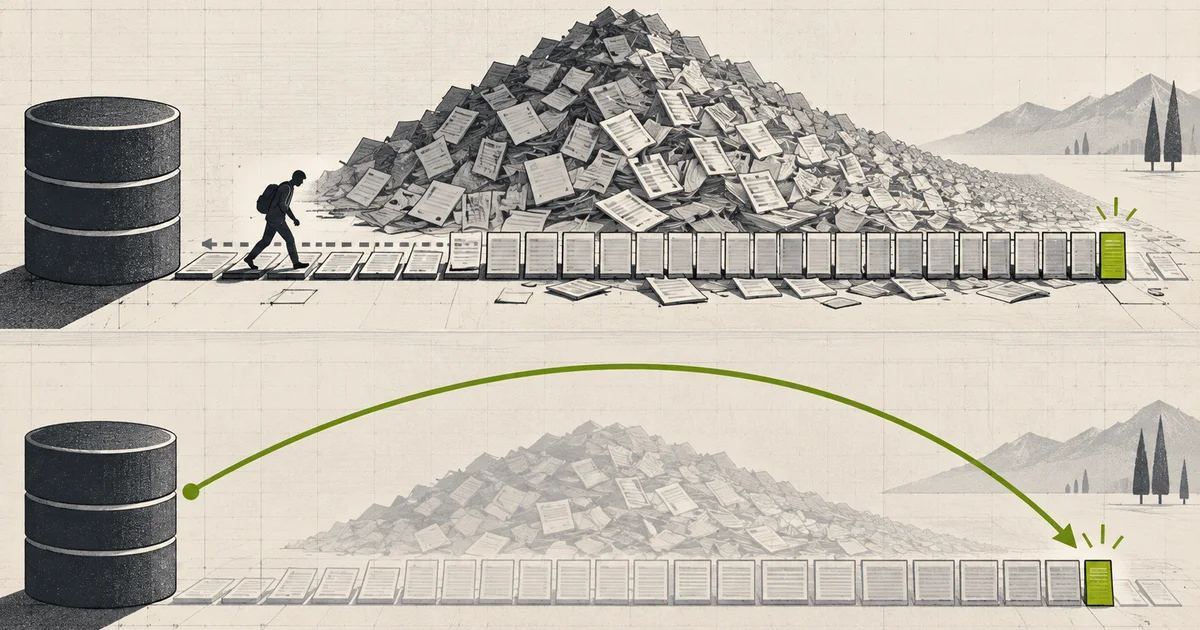
OFFSET Pagination: The Query That Gets Slower the Deeper You Scroll
OFFSET makes the executor process and discard rows before the page, so deep pages grow linearly even with an index. Keyset pagination bounds that work, and a unique tiebreaker makes the cursor unambiguous.
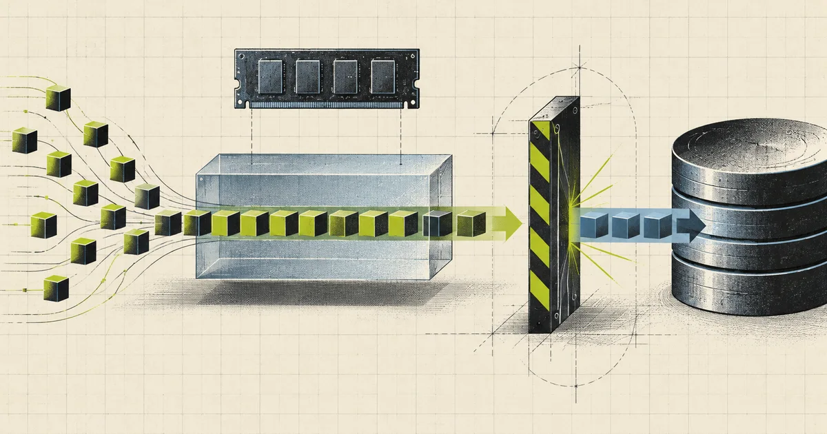
fsync: The Flush Between a Commit and Stable Storage
How PostgreSQL separates writes, WAL flushes, synchronous commit, hardware truthfulness, and group commit—and where each durability promise can fail.
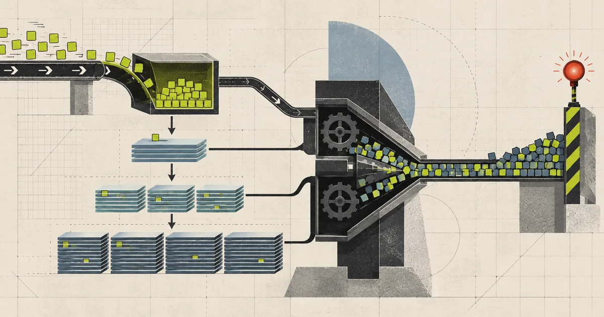
LSM Compaction: The Background Job That Becomes a Foreground Outage
Why an LSM engine saturates a disk with no user traffic, how write stalls turn a background merge into a latency incident, and why the disk needs headroom a capacity graph will never show.