Route Optimization Engine: The Problem That Looks Like a Shortest Path and Is Not

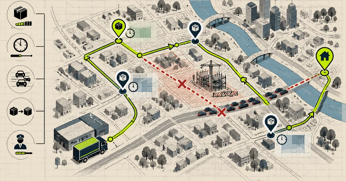
Every engineer building a route optimisation system starts by looking for a shortest-path algorithm, and every one of them discovers the same thing about forty minutes in: shortest path is one vehicle, one destination, no constraints, and the problem you have is a vehicle routing problem with capacity limits, time windows, and dozens of vehicles.

This article is about that problem, the algorithms that actually work on it, and the gap between the offline version you can solve optimally and the online version where a customer calls to add a stop at 4pm.

The scale, and what makes it hard

  a regional delivery operation
  20 vehicles
  300 stops per day
  15 stops per vehicle

  constraints
    - vehicle capacity: 60 parcels each
    - time windows: "deliver between 9:00 and 12:00"
    - service time: 4 minutes per stop
    - shift length: 8 hours
    - driver break: 30 min, once
    - max route duration: 7 hours

  decision variables
    which vehicle takes which stops
    in what order
    -> 15^20 orderings, roughly

The complexity statement that matters: the vehicle routing problem is NP-hard, and the practical sizes here are well past the point where exact methods help. A 20-vehicle, 300-stop problem has an astronomical number of candidate solutions, and the gap between the best known solution and a good heuristic solution is typically under 5% — which means the last hour of optimisation buys almost nothing compared to the first thirty seconds.

That is the key strategic fact. You are not building an exact solver. You are building a good-enough solver that runs fast enough to replan.

The three-layer architecture

  +----------------------------------------------------------+
  |  LAYER 3: metaheuristic (LNS, annealing)                  |
  |  escape local optima, ruin and recreate                   |
  |  5-60 seconds                                             |
  +----------------------------+-----------------------------+
                               |
                               v
  +----------------------------------------------------------+
  |  LAYER 2: local search                                    |
  |  improve the current solution in place                    |
  |  2-opt, Or-opt, relocate, swap, 2-opt*                    |
  |  milliseconds per pass, thousands of passes               |
  +----------------------------+-----------------------------+
                               |
                               v
  +----------------------------------------------------------+
  |  LAYER 1: construction                                     |
  |  build a feasible solution from nothing, fast             |
  |  greedy insertion, cheapest insertion, Clarke-Wright       |
  |  milliseconds                                            |
  +----------------------------------------------------------+

Three layers because each solves a different problem.

Construction must produce a feasible solution in milliseconds, because it runs on every replan and sometimes on every new order. A nearest-neighbour plus insertion heuristic will do this reliably. Its output is poor — typically 20-30% above optimal — and that does not matter, because layer 2 immediately improves it.

Local search improves the current solution with moves that keep feasibility. The core catalogue:

  relocate      move one stop to a different position
  swap          exchange two stops between routes
  2-opt         reverse a segment, removes route crossings
  Or-opt        move a segment of 2-3 stops
  2-opt*        exchange route tails between vehicles

The insight behind 2-opt is that the most common geometric pathology in a bad route is crossing edges — two route segments that intersect. Reversing the segment between the crossings removes both crossings and always shortens the route, so it is a strictly improving move with no objective evaluation needed. Removing crossings is a large fraction of the achievable improvement, which is why 2-opt is the first move implemented and the one that gets run most.

Metaheuristics are what stop you being stuck. Local search converges to a local optimum — no single improving move exists — and the only way out is to make a worse solution temporarily and see where it leads. Large neighbourhood search does this structurally:

  LNS, one iteration
    1. select a subset of stops
       (random, or by relatedness: spatially
        close, same time window, same customer)
    2. REMOVE them, keeping the rest fixed
    3. REINSERT them optimally or greedily
    4. keep the result only if it is better
       (or with small probability, accept anyway)

  repeat for the time budget

The removal strategy matters more than anything else in the whole algorithm. “Remove a random 20% and try to put it back” is the version that plateaus early. “Remove all stops in a geographic cluster and reinsert” and “remove all stops for one customer and reinsert” escape far more local optima, because they target the specific structures that are stuck — a cluster of nearby stops that got assigned to two different vehicles when one vehicle could serve them all.

Simulated annealing, and why accepting worse matters

  hill climbing
    accept a move only if it IMPROVES
    -> stuck at the first local optimum
    -> a route with 2 crossings that cannot
       be fixed by any single 2-opt move
       stays broken forever

  simulated annealing
    accept a move if it improves
    OR with probability exp(-delta / T)
    where T starts high and decays
    -> early: accepts almost anything, explores
    -> late: accepts almost nothing, exploits
    -> the "accept worse" phase is where the
       good solutions come from

The temperature schedule is a real parameter. Too high and the search random-walks for most of the budget; too low and it is hill climbing with extra steps. A geometric decay from an initial temperature set relative to the typical move cost, over the available time budget, is the standard answer.

Ruin-and-recreate is the same idea with a different mechanism, and it is generally more effective for vehicle routing because it uses problem structure rather than a random walk. A ruin operator that removes a whole customer across many vehicles, followed by a recreate that reinserts them properly, can move work between vehicles in a way that thousands of pairwise local moves never will. The pairwise moves are local in space; the ruin-recreate step is local in assignment, and that is the dimension where the real improvements live.

The cost matrix, and why the real problem is the travel times

  naive
    300 stops x 300 stops = 90,000 pairs
    call the routing API for each
    at 30ms each
    = 45 minutes

  that is not an option

  practical
    1. static distance matrix, precomputed
       from cached road network data
    2. travel time matrix, precomputed
       by time-of-day bucket
       (4 buckets x 90,000 pairs = 360,000 rows)
    3. refine dynamically for the stops
       in the current candidate routes

The matrix precomputation is a genuine design decision, not a detail. With a static matrix you can precompute once and reuse, but the numbers are only as good as the traffic assumptions baked in — a matrix built for 10am is wrong for 4pm, and optimising routes against morning travel times produces a plan that falls apart in the afternoon.

The middle option — time-of-day buckets — is what most production systems use, and it is a genuine improvement over a single matrix for a modest storage cost. Four or eight buckets is usually enough to capture the difference between peak and off-peak, and the accuracy gain is significant.

The dynamic refinement step is what keeps the final plan realistic: take the routes in the current best solution, recompute their actual travel times with live traffic, and use those in the objective. This makes each iteration slightly more expensive and the final answer substantially more truthful, and it is the difference between an optimiser that produces a good plan and one that produces a plan that survives contact with the afternoon.

Time windows are the constraint that dominates everything

  feasible solution requirement:
    every stop arrives within [open, close]
    capacity never exceeded
    shift never exceeded
    breaks respected

  if the construction heuristic cannot
  produce a feasible solution, it is useless

Time windows are harder than capacity because they make the problem potentially infeasible, and a router that cannot find a feasible solution has nothing to optimise. Three practical responses:

Cheapest insertion with feasibility checking. When inserting a stop, try every position in every route and take the first that keeps everything feasible. This is O(stops × routes × positions), which is expensive, and it is the only version of insertion that reliably finds a feasible solution when one exists.

Allow infeasible intermediate solutions during construction, then repair. Build a solution that violates time windows, let local search fix them, and treat the violation as a heavily weighted penalty in the objective. This is the standard approach in the research literature and it works better than strict insertion because it does not get stuck refusing to insert a stop that a later rearrangement would make feasible.

Recognise that infeasibility is often real. If a time window cannot be served by any vehicle, no algorithm will fix it. The right response is to detect it, report it to dispatch, and let a human decide — reschedule, reassign to a different operation, or notify the customer. An optimiser that silently drops the infeasible stop has made a business decision without telling anyone.

The online problem: replanning without breaking promises

The offline version of this problem is solved once per day. The online version is where the engineering actually is.

  what changes during the day
    - new orders arrive (constant)
    - a vehicle finishes early, finishes late
    - traffic diverges from the estimate
    - a vehicle breaks down
    - a customer is not available
    - a driver takes their break late

  what is already committed
    - customers have been told a delivery window
    - drivers have been given a stop list
    - some stops are already done

This is the constraint that shapes the design. You cannot recompute from scratch every time something changes, because the previous plan has been communicated to humans and a plan that changes every fifteen minutes is unusable by the people executing it.

The workable approach:

  plan horizon
    - full replan (e.g. nightly or early morning)
      optimises the whole day
    - rolling replan every 15-30 min
      optimises only the REMAINDER
      locks completed and in-progress stops
    - micro-replans for single events
      (new order, breakdown) -> cheapest
      insertion into the current plan,
      NOT a full optimisation

  the rule
    a full replan is allowed to change anything
    not yet started
    a micro-replan changes as little as
    possible to accommodate the change

That distinction — full replan versus micro-replan — is the single most important design decision in the whole system. Full replanning is where cost savings come from and where the instability comes from. A system that full-replans on every new order will produce a plan that is locally better and globally incomprehensible, and the drivers will stop trusting it.

A useful constraint on rolling replans: limit the amount of change allowed. If the new plan reorders more than N stops, do not take it, regardless of its cost. This is a deliberate cap on optimisation in exchange for a plan humans can execute, and it should be a number you can tune and a number you can explain.

ETAs and the prediction problem underneath

  route optimised against travel time T_estimate
  driver arrives at T_actual
  T_actual - T_estimate is the error

  error sources
    - static matrix vs live traffic
    - time-of-day bucket granularity
    - service time variance
        (the 4-minute estimate when the
         customer needs 12)
    - parking and walking time, not in
      the travel time at all
    - the driver's own knowledge
      (a local driver beats the algorithm
       on the same route)

Two things follow that are worth stating because they change what you optimise.

Service time variance is often larger than travel time variance. If you estimate 4 minutes per stop and the actual distribution is mean 5 with a long tail, the tail accumulates: 15 stops at an average of 2 extra minutes is 30 minutes of drift by the end of the route. Reducing the variance in service time estimates is worth more than improving the travel time model.

Predictability beats accuracy. A driver who is consistently 10 minutes late is a manageable problem. A driver who is sometimes 20 minutes early and sometimes 25 minutes late is not, because the customer-facing promise has to be a range and a wide range is a broken promise. This means the objective should sometimes prefer a plan that is robustly 12% worse over one that is optimally 5% worse but highly variable — which is a constraint, not an objective, and it is a real design decision.

Failure stories worth testing

Add 300 stops all in one 30-minute time window in a different postcode

Confirm the solver reports infeasibility rather than silently dropping stops. This is the test that distinguishes an optimiser from a lookup table.

Set a 30-second budget and compare against 5 minutes

Measure the cost difference. If it is under 3%, the short budget is the right operating point and the long one is waste. If it is 15%, the solver is not converging and there is a bug.

Run only 2-opt with no ruin-and-recreate

Confirm the solution plateaus well above what LNS reaches. This is the test for “we forgot the metaheuristic layer”.

Use a removal strategy of pure random in LNS

Compare against geographic-cluster removal. The difference is typically 5-10% and it is the cheapest optimisation available.

Use a static travel time matrix built at 10am and run at 4pm

Measure the arrival error. This is the test that shows why time-of-day buckets exist.

Add a vehicle breakdown at 11am

Confirm the stops transfer with minimal disruption and that the customer-facing windows still hold where possible. This tests the micro-replan path specifically.

Add 20 new orders in 10 minutes

Confirm the system does not full-replan each time. Watch the number of changed stops per replan — if it is large, drivers will stop following the plan.

Force a rolling replan that improves cost by 8% but reorders 40 stops

Confirm the change cap rejects it. This is the test for whether the stability constraint is real or aspirational.

Make service time estimates 3x too low

Measure the end-of-route drift. The test for whether service time variance is in your model at all.

Run with a driver who knows the area versus one who does not

Measure the ETA error difference. If a local driver’s routes are consistently shorter, your travel time model is missing something the driver has, and that is a modelling question.

Solve a plan and then execute it manually with realistic service times

Measure the actual completion against the plan. This is the only test that validates the whole chain, and it is the one that surprises people.

A production-ready architecture

   constraints input
     - stops, windows, service times
     - vehicles, capacity, shifts, breaks
     - traffic time-of-day matrix
        |
        v
  +----------------------------------------------------------+
  |  L1 construction                    < 1s                 |
  |  cheapest-insertion with feasibility check               |
  |  fallback: greedy + repair                             |
  +----------------------------+-----------------------------+
                               |
                               v
  +----------------------------------------------------------+
  |  L2 local search                   seconds               |
  |  relocate, swap, 2-opt, Or-opt, 2-opt*                   |
  |  first-improvement with don't-look bits                  |
  |  dynamic travel-time refinement for candidate routes      |
  +----------------------------+-----------------------------+
                               |
                               v
  +----------------------------------------------------------+
  |  L3 ruin and recreate / LNS        5-60s                 |
  |  removal: geographic, customer, time-window related      |
  |  recreate: greedy reinsert, accept if better             |
  |  or accept-worse with small probability (annealing)      |
  +----------------------------+-----------------------------+
                               |
             time budget reached, solution is feasible
                               |
                               v
  +----------------------------------------------------------+
  |  change guard                                            |
  |  - lock completed / in-progress stops                   |
  |  - cap the number of changed stops per replan            |
  |  - full replan nightly, rolling every 15-30 min,         |
  |    cheapest-insertion for single events                 |
  +----------------------------+-----------------------------+
                               |
                               v
  +----------------------------------------------------------+
  |  execution + feedback                                    |
  |  driver app, actual service times, actual ETAs          |
  |  feed back: service time distribution, driver variance,  |
  |  predicted vs actual                                     |
  +----------------------------------------------------------+

  watch: feasibility failures, cost vs baseline,
         predicted vs actual ETA, change rate per replan

A sensible delivery checklist:

1. Build in three layers — construction, local search, ruin-and-recreate — and budget the time explicitly. Most systems need 30 seconds, not 30 minutes.
2. Implement 2-opt first. Removing crossing edges is the largest share of achievable improvement for the least code.
3. Choose the LNS removal strategy deliberately. Geographic and customer-cluster removal beat random by a wide margin.
4. Accept worse solutions sometimes. An optimiser that only accepts improvements stops at the first local optimum.
5. Precompute the cost matrix with time-of-day buckets, and refine dynamically for candidate routes in the current solution.
6. Treat infeasibility as a result to report, not an error to swallow. A stop that cannot be served is a business decision.
7. Model service time as a distribution, not a constant. The tail accumulates faster than the travel time error.
8. Separate full replanning from micro-replanning, and make the difference explicit in the API.
9. Cap the number of stops a replan may change. A plan humans can execute beats a plan that is 8% cheaper.
10. Feed actual service times and actual ETAs back into the model, and measure predicted against actual continuously.
11. Optimise for predictability as well as cost. A consistent 10% overrun is more manageable than a variable one.
12. Keep a baseline solution from before the optimiser existed. “The optimiser made it 12% cheaper” is only meaningful against a number.

Common mistakes

Mistake	What actually happens	Better decision
Using a shortest-path solver	Solves one vehicle, no constraints	A VRP solver with move operators
Exact methods at real scale	Never finishes, or a very weak bound	Heuristics; the optimality gap is under 5%
Local search only	Stuck at the first local optimum	Ruin-and-recreate, or annealing
Random removal in LNS	Plateaus early, 5-10% worse	Geographic and customer-cluster removal
Never accept a worse solution	No escape from local optima	Accept-worse with decaying probability
Single static travel time matrix	Optimising against the wrong traffic	Time-of-day buckets, dynamic refinement
Ignoring service time variance	End-of-route drift of 30+ minutes	Model it as a distribution
Feasibility checked after optimisation	Infeasible plans returned as valid	Check during construction, or repair
Silently dropping infeasible stops	A business decision made by a solver	Report to dispatch, let a human decide
Full replan on every new order	Plan changes constantly, drivers ignore it	Micro-replan for single events
No change cap on replans	Locally better, globally unusable	Cap changed stops, tune and explain it
Optimising in the abstract and driving in reality	Plan survives 4 hours	Measure predicted vs actual continuously
Ignoring driver local knowledge	Model is wrong where drivers are right	Learn from actual routes, not just the map
No baseline comparison	“12% better” than what is unclear	Keep the pre-optimiser solution as a baseline
Same objective for a 300-stop and 30-stop run	Small instances get the same budget as large	Budget by instance size and deadline
Assuming more optimisation time helps	Diminishing returns past ~60s	Measure the time-quality curve, pick the knee
Single vehicle type	Capacity and shift ignored	Vehicle types as constraints
No deadhead cost	Depot travel is free in the model	Include return-to-depot and reload logic
Break time not modelled	Routes that cannot be driven legally	Breaks as hard constraints with windows
Trusting the solver’s cost breakdown	Never reconciled with actuals	Reconcile planned versus executed time

The complete story in one minute

Shortest path is one vehicle, one destination, no constraints. What you actually have is a vehicle routing problem with capacity, time windows, and dozens of vehicles, which is NP-hard. The useful fact is that the gap between a good heuristic and the best known solution is typically under 5%, so the goal is not optimality — it is a solver good enough that you can replan every few minutes.

Three layers, each solving a different problem. Construction produces a feasible solution in milliseconds, because it runs on every replan. Local search improves it with 2-opt, Or-opt, relocate, and swap, where 2-opt earns its place because removing crossing edges is a large share of the achievable gain with almost no code. Metaheuristics on top escape the local optima, and the crucial property is that they accept worse solutions temporarily — hill climbing stops at the first local optimum, which is often a route with two crossings that no single move can fix. Ruin-and-recreate is more effective than annealing here because it operates on assignment, which is the dimension where the real improvements live.

The objective is not the hard part. The hard part is the travel times: a matrix built for 10am is wrong for 4pm, so precompute with time-of-day buckets and refine dynamically for the candidate routes in the current solution. And service time variance accumulates faster than travel time error, which is why a long-tailed 4-minute estimate produces 30 minutes of drift by stop fifteen.

In production, everything is shaped by one constraint: the previous plan has already been promised to drivers and customers. Full replans optimise the whole day, rolling replans optimise only the remainder with completed stops locked, and a new order triggers cheapest insertion rather than a full optimisation. Cap how many stops a replan may reorder, deliberately, and accept less cost for a plan humans can execute.

construct fast, improve locally, escape with ruin-and-recreate
time-of-day cost matrix, dynamic refinement, service time as a distribution
full replan / rolling replan / micro-replan, with a change cap
accept a worse solution now to find a better one later

The hard part was never finding the shortest path between two points. It was keeping a plan stable enough for a human to execute while the traffic changes underneath it.

What this team still owns

The solver owns neither truth nor operations. The product team owns the constraint model, matrix freshness, solve deadline, infeasibility response, and stability penalty between successive plans. Persist objective components and violated soft constraints with each solution. Re-optimise only the affected horizon, freeze work already accepted or underway, and make “no feasible solution” a supported result; inventing a route that violates a legal or customer window is not graceful degradation.

Technical references

• Google OR-Tools: vehicle routing
• Google OR-Tools: search limits
• Google Maps Route Optimization API: time windows